Optimization Fundamentals in Machine Learning: The Engine Behind Every Model

Before a model can learn, it needs two things: a way to measure how wrong it is, and a mechanism to become less wrong over time.

That’s optimization — and it’s the engine quietly running under every model you’ll ever train.

Most tutorials introduce you to an algorithm, show you a .fit() call, and move on. The model trains. The accuracy goes up. Everything seems fine. But when something breaks — and it will — you need to understand what’s actually happening inside that training loop. When your model isn’t converging, when your loss is bouncing all over the place, when training is glacially slow, the answer is almost always here.

This post exists so that when we get to individual algorithms in future posts, you’re never confused about why they work the way they do. Optimization is the shared foundation. Know it once; apply it everywhere.

No formula-dropping without context. No assumed prerequisites. Let’s build this from the ground up.

The Core Problem: What Does “Learning” Actually Mean?

Here’s a thing that doesn’t get said plainly enough:

A machine learning model is just a mathematical function with adjustable knobs. Training is the process of turning those knobs until the function produces outputs close to what you want.

Those knobs? They’re called parameters — the weights and biases inside a model. At the start of training, they’re set randomly. They produce garbage outputs. The job of optimization is to systematically adjust them until the outputs are good.

But “good” needs a definition. You can’t adjust toward a goal you haven’t specified. That’s where the loss function comes in.

The Loss Function: How Wrong Are You, Exactly?

A loss function (also called a cost function or objective function) takes the model’s prediction and the actual correct answer, and returns a single number that represents the error. The higher the number, the worse the model is doing.

The goal of training is to find parameter values that make this number as small as possible.

💡 The loss function is the definition of success. Whatever it measures, that’s what the model will optimise toward — for better or worse. Choosing the wrong loss function is one of the most impactful mistakes you can make, and it’s surprisingly common.

The Most Common Loss Functions

Loss Function	Full Name	Used For	Intuition
MSE	Mean Squared Error	Regression	Average of squared differences between prediction and truth
MAE	Mean Absolute Error	Regression (robust)	Average of absolute differences; less sensitive to outliers
Binary Cross-Entropy	Log Loss	Binary Classification	Penalises confident wrong predictions severely
Categorical Cross-Entropy	Multiclass Log Loss	Multi-class Classification	Extends binary cross-entropy to multiple classes
Hinge Loss	—	SVMs	Maximises the margin between classes

MSE vs MAE: The Outlier Sensitivity Trade-off

Both measure prediction error in regression. The difference is in how they handle extremes.

MSE squares each error before averaging. A prediction that’s off by 10 contributes 100 to the loss. A prediction off by 100 contributes 10,000. Squaring amplifies large errors dramatically — which means MSE “cares more” about getting the big mistakes right. Useful when large errors are genuinely unacceptable.

MAE takes absolute values, not squares. An error of 10 contributes 10. An error of 100 contributes 100. The relationship is linear. This makes MAE far more robust when your data has outliers you don’t want disproportionately affecting the model.

🚨 The myth: MSE is always better because it’s mathematically convenient.

MSE has nice mathematical properties (smooth, differentiable everywhere) which makes gradient computation easier. But “mathematically convenient” ≠ “right for your problem.” If your dataset has meaningful outliers — real extreme values you want the model to learn from without being dominated by — MAE often produces better models. Choose based on the problem, not the convention.

Why Cross-Entropy for Classification?

For classification, you might wonder: why not just count wrong predictions? Why this more complex formula?

Because counting wrong predictions throws away useful information. A model that’s 51% confident about the wrong class and a model that’s 99% confident about the wrong class are both “wrong” in a count — but they’re very different situations.

Cross-entropy penalises confident mistakes much more heavily than uncertain ones. If your model predicts 99% probability for the wrong class, the loss spikes severely. If it predicts 51% for the wrong class, the loss is relatively small. This pushes models to be both accurate and well-calibrated in their confidence.

The Loss Landscape: Visualising the Problem

Here’s a mental model that will stick with you forever.

Imagine a hilly landscape — mountains, valleys, flat plateaus. Your model’s current parameter values correspond to a specific location on this landscape. The height at any location is your loss. Your goal: find the lowest point (the valley).

This is called the loss landscape, and optimisation is the problem of navigating it.

Loss Landscape Graph

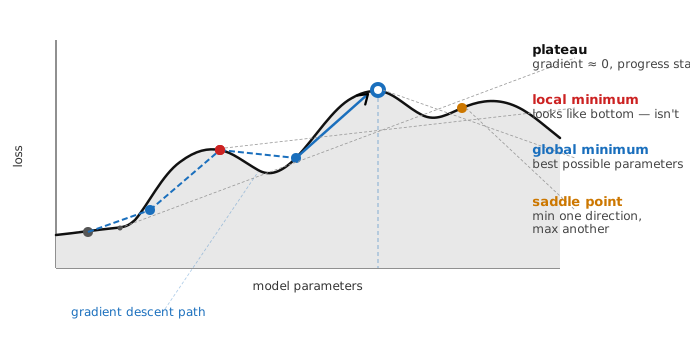
The landscape can have:

Global minimum — the absolute lowest point; the best possible parameters
Local minima — valleys that aren’t the lowest, but look like it from nearby
Saddle points — a location that’s a minimum in one direction but a maximum in another
Plateaus — flat regions where the gradient is nearly zero and progress is painfully slow

The question optimisation algorithms answer: how do you navigate this landscape efficiently without getting stuck?

The most fundamental optimisation algorithm in all of machine learning is gradient descent. Everything else — Adam, RMSProp, AdaGrad — is a refinement of this core idea.

The intuition is elegant:

If you’re standing on a hill and want to get to the bottom, look at the slope beneath your feet and take a step downhill. Repeat.

In mathematical terms, the gradient is a vector that points in the direction of steepest increase in the loss. So to minimise the loss, you move in the opposite direction — downhill.

At each step:

new_parameters = old_parameters − (learning_rate × gradient)

That’s it. That’s gradient descent. The sophistication in modern optimisation is entirely about how you compute the gradient and how you take the step — but this update rule is the skeleton.

💡 Why “descent”? You’re descending the loss landscape. The gradient points uphill; you go the other way. Step by step, iteration by iteration, you find your way toward a minimum.

The Learning Rate: The Most Important Knob You Have

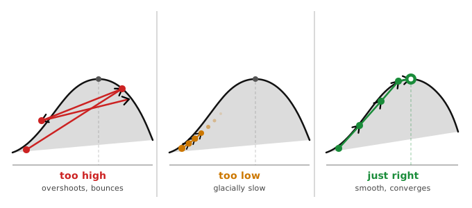
The learning rate controls how big each step is in gradient descent. It’s a small number — typically between 0.0001 and 0.1 — and it has an outsized effect on training.

Learning Rate	What Happens
Too high	Steps are too large; you overshoot the minimum and bounce around or diverge
Too low	Steps are tiny; training is very slow; you may get stuck early
Just right	Smooth, steady descent toward the minimum

Learning Rate

Learning Rate Schedules: Adapting Over Time

A fixed learning rate is rarely optimal. Early in training, you want larger steps to explore the landscape quickly. Later, when you’re close to a minimum, you want smaller steps to converge precisely without bouncing past.

Learning rate schedules reduce the learning rate as training progresses:

Step decay — reduce by a fixed factor every N epochs (e.g., halve every 10 epochs)
Exponential decay — continuously shrink at an exponential rate
Cosine annealing — smoothly oscillate between a high and low learning rate
Warmup + decay — start small, ramp up, then decay (common in transformer training)

💡 In practice: If you’re using modern optimisers like Adam (discussed below), the learning rate matters less than in vanilla gradient descent — Adam adapts the effective rate per parameter automatically. But it still matters enough to tune.

A Note on Optimisers

Vanilla gradient descent is the foundation, but in practice you’ll rarely use it in its pure form. Modern optimisers like SGD with Momentum, RMSProp, and Adam build on the same core idea — move opposite to the gradient — but add smarter mechanics: adaptive learning rates per parameter, accumulated velocity, noise resistance.

💡 The one thing to know for now: When you open a library like PyTorch or Keras and need to pick an optimiser, start with Adam. It’s robust, requires minimal tuning, and works well across most problems. The full breakdown of how these optimisers differ, when to switch, and what’s happening under the hood gets its own dedicated post.

Epochs, Iterations, and Convergence

Three terms you’ll see constantly:

Epoch — one complete pass through the entire training dataset
Iteration — one parameter update step (one mini-batch processed)
Convergence — the point at which the loss stops decreasing meaningfully

If you have 10,000 samples and a batch size of 100, one epoch = 100 iterations.

How Many Epochs?

There’s no universal answer, and anyone who gives you a specific number without context is guessing. The right number of epochs depends on:

Model complexity
Dataset size
Learning rate
Whether you’re using early stopping

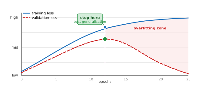
Early stopping is the practical solution: monitor validation loss during training and stop when it stops improving (or starts getting worse). This prevents overfitting from over-training and removes the “how many epochs?” guessing game.

Earlt Stopping

The Vanishing and Exploding Gradient Problems

For completeness — and because you’ll hit these — two notorious problems in deep network training:

Vanishing Gradients

As gradients flow backward through many layers (via backpropagation, which we’ll cover in depth separately), they can become exponentially small. By the time they reach the early layers, they’re essentially zero. Those layers stop learning entirely.

This was the main reason deep networks were considered untrainable before ~2010. Solutions: better weight initialisation, ReLU activation functions, batch normalisation, residual connections (skip connections).

Exploding Gradients

The opposite: gradients grow exponentially as they propagate backward, eventually becoming NaN (not-a-number). Training collapses.

Solution: gradient clipping — if the gradient magnitude exceeds a threshold, scale it down to that threshold. A simple fix that works well in practice.

🚨 Symptom you’ll recognise: If your loss suddenly jumps to nan during training, exploding gradients are a likely culprit. Reduce your learning rate or add gradient clipping.

Regularisation: Keeping Optimisation Honest

There’s a problem with pure loss minimisation: the model can find parameters that make the training loss very low by memorising the data rather than learning its patterns. The loss function doesn’t know the difference — it just sees a low number.

Regularisation adds a penalty to the loss for overly complex parameters, discouraging memorisation and encouraging generalisation.

L2 Regularisation (Weight Decay)

Adds the sum of squared parameter values to the loss. Large parameter values become expensive. The optimiser is pushed to find small, distributed weights rather than a few extreme ones.

Total Loss = Data Loss + λ × (sum of squared weights)

λ (lambda) controls how strong the penalty is. Higher lambda = stronger push toward simplicity.

L1 Regularisation (Lasso)

Adds the sum of absolute parameter values. Unlike L2, L1 tends to push many weights exactly to zero — effectively performing feature selection by eliminating irrelevant parameters entirely.

Regularisation	Effect	Use When
L2 (Ridge)	Shrinks weights toward zero; keeps all features	Default for most models
L1 (Lasso)	Pushes many weights to exactly zero	Feature selection desired
Dropout	Randomly deactivates neurons during training	Neural networks
Early stopping	Stops training before overfitting	Always — a free regulariser

💡 Dropout deserves a special mention. Used in neural networks, it randomly “turns off” a fraction of neurons during each training step. This forces the network to not rely on any single neuron, developing more robust, distributed representations. At inference time, all neurons are active (with their weights scaled accordingly). It’s one of the most effective regularisers for deep networks — and one of the cleverest ideas in the field.

The Full Training Loop, Demystified

Put everything together, and here’s what happens every time you call .fit():

For each epoch:
  └── For each batch of data:
        1. FORWARD PASS
           Feed batch through model → get predictions
        
        2. COMPUTE LOSS
           Compare predictions to true labels using loss function
           Add regularisation penalty (if any)
        
        3. BACKWARD PASS (Backpropagation)
           Compute gradient of loss with respect to every parameter
        
        4. CLIP GRADIENTS (optional)
           If gradient magnitude > threshold, scale it down
        
        5. UPDATE PARAMETERS
           new_params = old_params − (lr × gradient)
           (or the adaptive equivalent for Adam/RMSProp)
  
  └── After each epoch:
        6. EVALUATE on validation set
        7. Check early stopping criterion
        8. Adjust learning rate (if using a schedule)

Every training run you’ll ever do — simple linear regression to billion-parameter transformers — is a version of this loop.

Common Failure Modes and What They Mean

Symptom	Likely Cause	What to Try
Loss not decreasing at all	Learning rate too low; bad initialisation; vanishing gradients	Increase LR; check architecture; use better initialisation
Loss bouncing wildly	Learning rate too high	Reduce LR; add LR schedule
Loss → `nan`	Exploding gradients; numerical instability	Gradient clipping; reduce LR
Loss decreasing but val loss increasing	Overfitting	Add regularisation; early stopping; more data
Training fast initially, then stuck	Hit a saddle point or plateau	Momentum; adaptive optimiser; LR warmup
Training and val loss both plateau early	Underfitting	More complex model; more epochs; higher LR

Quick Reference

Term	One-Line Definition
Loss Function	Measures how wrong the model’s predictions are
Gradient	Vector pointing in direction of steepest loss increase
Gradient Descent	Iteratively move opposite to gradient to reduce loss
Learning Rate	Step size per gradient descent update
Epoch	One full pass through the training dataset
Convergence	When the loss stops meaningfully decreasing
Adam	Modern adaptive optimiser; the practical default for most training
L1 / L2 Regularisation	Penalty on large weights to prevent overfitting
Early Stopping	Stop training when validation loss stops improving
Vanishing Gradient	Gradients shrink to near-zero in deep layers; learning stops
Exploding Gradient	Gradients grow unboundedly; training collapses
Loss Landscape	Conceptual surface where height = loss; training navigates it
Backpropagation	Algorithm to compute gradients efficiently through a network