Data Fundamentals for Machine Learning: The Complete Beginner’s Guide

Data Fundamentals of Machine Learning

There’s a quiet assumption baked into most ML tutorials: that you already know what “data” means in this context. Not rows in a spreadsheet. Not a CSV you downloaded. Something structured, shaped, cleaned, and split in a very particular way — and if you skip understanding that, every algorithm you learn later will feel like it’s floating in the air with no ground beneath it.

This post is about putting ground under your feet.

We’ll walk through the essential vocabulary and ideas — not as a glossary to skim and forget, but as a connected story. By the end, when the next posts get into models and training, you’ll already have the mental scaffolding to follow along without hitting a wall every three paragraphs.

No assumptions. No skipped steps. Let’s go.

What Is Data in ML, Really?

In everyday language, “data” means information. In machine learning, it means something more specific:

A collection of observations, each described by a set of measurable properties, often with a known outcome attached.

Let’s make this concrete with a real scenario.

Say you’re building a model to predict whether a loan applicant will repay their loan. Here’s how the ML vocabulary maps to that:

ML Term	What It Means	Loan Example
Observation	One individual record (also: sample, example, data point)	One loan applicant
Feature	A measurable property used as input	Age, income, credit score
Label	The outcome the model is predicting (also: target, output)	Repaid: Yes / No
Dataset	The full collection of observations	All past applicants

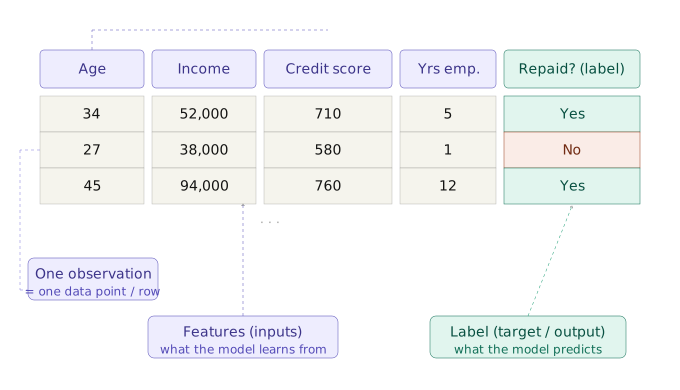
So a dataset is essentially a table. Each row is one observation. Each column except the last is a feature. The last column is the label:

| Age | Income | Credit Score | Years Employed | Repaid? |
|-----|--------|--------------|----------------|---------|
|  34 | 52000  |     710      |       5        |   Yes   |
|  27 | 38000  |     580      |       1        |   No    |
|  45 | 94000  |     760      |      12        |   Yes   |

Simple table. But there’s a lot of thinking packed into how you build it, clean it, and hand it to a model. That’s what this entire post unpacks.

Dataset Anatomy

Features: Not All Inputs Are Created Equal

Features are the raw material of learning. The model has no eyes, no intuition, no common sense — it can’t look at an applicant and form an impression. All it has is numbers and categories, and it learns entirely from those.

The quality, relevance, and form of your features determine the ceiling of how good a model can ever be. No algorithm, however sophisticated, rescues a dataset with bad or irrelevant features.

Features come in three types, and knowing which type matters:

🔢 Numerical Features

Quantities you can measure on a scale.

Continuous — can take any value in a range: weight (70.3 kg), temperature (36.8°C), time spent on page (47.2 seconds)
Discrete — counted whole numbers: number of children (2), missed payments (3), visits to a store (7)

🏷️ Categorical Features

Membership in a category with no inherent numeric meaning.

Job type: salaried / self-employed / unemployed
City: Mumbai / Delhi / Bangalore
Loan purpose: home / car / education

The model can’t do math on the word “Mumbai” — these need conversion before training. (More on this in the encoding section.)

📊 Ordinal Features

Categories with a meaningful order, but unequal gaps between them.

Education: high school < bachelor’s < master’s < PhD
Satisfaction rating: Poor < Average < Good < Excellent

The order matters, but you can’t say a master’s degree is “exactly twice” a bachelor’s the way 40°C is exactly twice 20°C. This distinction matters when you decide how to encode them.

💡 Quick Rule of Thumb Ask yourself: “Does the distance between values mean something?” If yes → numerical. If there’s order but distance is unclear → ordinal. If there’s neither → categorical.

Labels: What the Model Is Learning Toward

The label is the “right answer” the model is trying to approximate. And depending on what kind of label you have, your entire approach to ML shifts.

Label Type	Task	Examples
Category (finite set of classes)	Classification	Spam / Not Spam · Disease / No Disease · Dog / Cat / Bird
Number (continuous value)	Regression	House price · Tomorrow’s temperature · Expected sales
No label at all	Unsupervised Learning	Customer segments · Anomaly detection

The Most Common Myth About Labels

“More label classes = harder problem.”

Not necessarily. Predicting which of 10 digits (0–9) a handwritten image shows can be easier than binary classification of whether a transaction is fraudulent — because fraud patterns are subtle, rare, and constantly evolving. The difficulty of classification depends far more on how separable the classes are in your data than on how many classes exist.

For now, the key takeaway: labeled data → supervised learning. No labels → unsupervised. Both are valid, both are widely used, and we’ll explore each in dedicated posts.

The Dataset Split: Train, Validation, and Test

Here’s a concept that trips up almost every beginner — and even catches experienced practitioners when they’re moving fast.

When a model trains, it learns by looking at examples. If you then evaluate how good it is on those same examples, you’ll get a misleadingly optimistic result. The model has essentially memorised them. It’s like practising on past year’s exam papers and being graded on that same paper. You’d score 100% — and understand nothing new.

The solution: hold out data the model never sees during training, and use that for evaluation.

The Three-Way Split

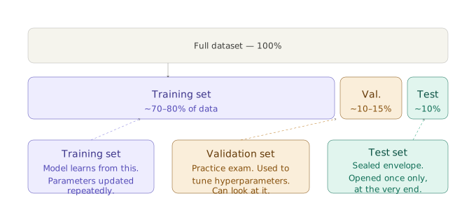
Your Full Dataset (100%)
│
├── Training Set   (~70–80%)  ← Model learns from this
├── Validation Set (~10–15%)  ← Used during tuning and development
└── Test Set       (~10–15%)  ← Locked until the very end

Training Set — Where learning happens. The model adjusts its internal parameters based on these examples, over and over, until it gets good at the task.

Validation Set — Your development feedback loop. When you’re adjusting settings (called hyperparameters — number of layers, learning rate, tree depth), you measure performance on the validation set to guide your decisions. It’s a practice exam you can look at.

Test Set — The sealed envelope. You open it once, after all decisions are made, to get your honest, final performance number. It simulates how the model will behave on data it has truly never seen.

⚠️ The Rule You Cannot Break

Data from the test set must never influence any training or tuning decision. Not even accidentally. If you peek at test performance to decide which model to keep, it’s no longer a test set — it’s a validation set with extra steps. Your final number is now optimistic and untrustworthy.

Train Vs Validation Vs Split

Overfitting and Underfitting: The Two Ways Models Fail

These two terms will appear in nearly every ML conversation. Understand them now and everything that follows will make more sense.

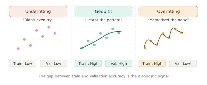
Overfitting — “Brilliant at school, useless in the real world”

The model has learned the training data too well — including its noise, quirks, and random patterns that don’t generalise. It gets near-perfect scores on training data and falls apart on new data.

Imagine a student who memorises every past exam question instead of understanding the subject. They’ll ace a repeated exam and bomb anything slightly different.

Signs: Training accuracy very high. Validation/test accuracy significantly lower.

Underfitting — “Didn’t even try”

The model is too simple to capture the actual patterns. It performs poorly on training data and poorly on new data.

Same student analogy: they showed up but didn’t study at all. No memorisation, no understanding.

Signs: Both training and validation accuracy are low.

Overfitting Vs Ideal Vs Underfitting

The Sweet Spot

	Training Performance	Validation Performance	Diagnosis
✅ Just right	High	Also high	Good generalisation
❌ Overfitting	Very high	Much lower	Too complex / too long trained
❌ Underfitting	Low	Low	Too simple / insufficient training

💡 This tension — between a model that memorises and one that generalises — is the central challenge of all of machine learning. Every regularisation technique, every architecture choice, every data augmentation strategy you’ll ever encounter is essentially an attempt to navigate it. Keep this framing in your head.

Data Quality: The Unglamorous Work Nobody Talks About Enough

Here’s a fact that surprises most people new to ML:

In real-world projects, data scientists spend 60–80% of their time on data — collecting, cleaning, and preparing it. Not on algorithms.

The algorithms are almost the easy part. The data is where the actual work lives.

The Four Data Quality Problems You Will Always Encounter

1. Missing Values

Sensors fail. Users skip fields. Systems crash mid-import. Missing data is the rule, not the exception.

What to do:

Drop the row — acceptable when very few rows are affected and you have enough data
Drop the feature — when a column is mostly empty (>50–60% missing is often a threshold)
Impute — fill in a sensible replacement:
- Numerical: mean (if no outliers), median (more robust), or a model-predicted value
- Categorical: most frequent value, or a dedicated “Unknown” category

🚨 Never impute before splitting your data. If you compute the mean on the full dataset (including your test set) and use it to fill missing values, you’ve leaked information from the test set into training. Always split first, then impute using statistics from the training set only.

2. Outliers

An age of 300. An income of ₹10 billion. A transaction amount of -99999.

Outliers can be real (a genuine extreme value in your data) or errors (bad entry, system glitch). Either way, they distort what a model learns — especially models that rely on distances or averages.

What to do: Investigate first. Remove if it’s clearly an error. Cap at a reasonable maximum (called winsorisation) if it’s real but extreme. Or use an algorithm that’s robust to outliers.

3. Duplicate Records

The same observation appearing twice inflates your training set and can cause the model to weight those examples more. In evaluation, duplicates shared between train and test sets will give you artificially inflated accuracy.

What to do: Deduplicate early, before the split.

4. Inconsistent Formatting

"Male", "male", "M", "MALE"  →  four values the model sees as different categories
"01/06/2024", "June 1, 2024"  →  two formats for the same date
"Mumbai", "Bombay"  →  same city, two names

What to do: Standardise. Pick a format, apply it uniformly. Build it into your data pipeline so incoming data gets the same treatment automatically.

Feature Scaling: Levelling the Playing Field

Here’s a subtle problem that catches a lot of beginners:

A dataset has two features — Age (values: 18–70) and Annual Income (values: ₹200,000–₹5,000,000). The income values are roughly 50,000× larger in raw magnitude.

For many algorithms, this creates a problem: the larger-scale feature dominates the learning process, simply because of its scale — not because it’s actually more important. The model effectively ignores age.

Feature scaling fixes this by rescaling numerical features to comparable magnitudes.

Two Methods — When to Use Which

Method	Formula	Result	Use When
Normalisation (Min-Max)	`(value − min) / (max − min)`	All values between 0 and 1	Algorithm expects bounded inputs (some neural networks)
Standardisation (Z-score)	`(value − mean) / std_deviation`	Mean = 0, Std = 1, no fixed range	General default; more robust to outliers

Does Every Algorithm Need Scaling?

No — and this is a common point of confusion.

Scale-sensitive (scaling required):

K-Nearest Neighbours — measures distance between points; unscaled features dominate
Support Vector Machines — distance-based decision boundaries
Logistic Regression / Linear Regression — gradient descent converges faster with scaling
Neural Networks — almost always benefit from scaling

Scale-invariant (no scaling needed):

Decision Trees — split on thresholds, not distances; magnitude doesn’t matter
Random Forests — same reason
Gradient Boosted Trees (XGBoost, LightGBM) — tree-based, scale-invariant

💡 When in doubt, scale. It never hurts tree-based models (they’ll just ignore it), and it can significantly help distance- and gradient-based ones.

Encoding Categorical Features: Teaching Numbers to Represent Words

Algorithms work with numbers. A column containing “Mumbai”, “Delhi”, “Bangalore” needs to become numerical before training.

There are two common approaches — and choosing the wrong one can silently hurt your model.

Label Encoding

Assign an integer to each category:

Mumbai    → 0
Delhi     → 1
Bangalore → 2

The problem: This introduces a false ordering. The model may interpret Bangalore (2) as “twice” Delhi (1), or “greater than” Mumbai (0) — which is meaningless for city names.

When it’s actually fine: For tree-based models, where splits are threshold-based and the model won’t treat the numbers as having a magnitude relationship. Also appropriate for genuinely ordinal features (Poor=0, Average=1, Good=2, Excellent=3 — where the order is real).

One-Hot Encoding

Create a separate binary column for each category:

           Mumbai  Delhi  Bangalore
Mumbai  →    1       0       0
Delhi   →    0       1       0
Bangalore →  0       0       1

The benefit: No false ordering. Each city is equidistant from every other.

The cost: The number of columns grows with the number of categories. 200 cities = 200 new columns. This can become a serious problem — known as high cardinality.

What About High-Cardinality Features?

This is one of those things tutorials rarely address but that comes up constantly in real data:

A feature with hundreds or thousands of unique values (postal codes, product IDs, user IDs) can’t realistically be one-hot encoded.

Solutions include target encoding (replace each category with the mean of the label for that category), frequency encoding (replace with how often the category appears), and embeddings (learn a dense vector representation — the same idea behind word embeddings in NLP). We’ll cover these in depth later.

Feature Distributions: The Shape of Your Data

The distribution of a feature describes how its values are spread across the range.

Understanding distributions isn’t just academic. It’s how you catch problems before they reach the model, and how you decide what transformations a feature needs.

Common Distribution Shapes and What They Signal

Shape	Description	Example Feature	What to Do
Normal (bell curve)	Symmetric around the mean	Height, measurement error	Usually fine as-is
Right-skewed	Long tail toward high values	Income, house prices, response times	Log-transform often helps
Left-skewed	Long tail toward low values	Test scores (if easy exam)	Square or cube transform
Bimodal	Two distinct peaks	Age of a product’s users (young & old)	Consider splitting into groups
Uniform	Flat, all values equally common	Random IDs	May not be a useful feature
Heavily zero-inflated	Most values are 0	Days since last purchase (many new users)	Treat as two features: is-zero flag + non-zero values

The Log Transformation in Practice

Income is a classic right-skewed feature — most people earn in a moderate range, but a small number earn extremely high amounts, creating a long rightward tail. This skew can distort model learning.

Applying a log transformation (log(income)) compresses the tail and brings the distribution closer to symmetric. The relative ordering is preserved — a higher income is still higher — but the extreme values no longer dominate.

One thing nobody tells you early: always visualise your features before doing anything else. A histogram of each feature takes five minutes and can save you hours of debugging mystery model behaviour downstream.

How Much Data Is “Enough”?

This is one of the most common questions from people starting out — and it has no clean answer. But there are useful frameworks.

The Real Factors That Determine Data Needs

Pattern complexity — A subtle pattern in a high-dimensional space needs more data to surface than an obvious one
Number of features — More features generally require more data (this is the curse of dimensionality)
Signal-to-noise ratio — Clean, consistent data goes further than noisy data
Algorithm complexity — More parameters = more data needed to avoid overfitting

Rough Order-of-Magnitude Intuitions

Model Type	Rough Data Requirement
Simple linear/logistic regression	Hundreds to low thousands
Tree-based models (RF, XGBoost)	Thousands to tens of thousands
Deep neural networks (tabular)	Tens of thousands+
Computer vision CNNs	Hundreds of thousands to millions
Large language models	Billions of tokens

⚠️ The myth: “More data always helps.”

Not if the additional data is noisy, mislabelled, or irrelevant. 10,000 high-quality, correctly labelled examples will outperform 1,000,000 poorly labelled ones. Data volume is not a substitute for data quality.

The more useful question isn’t “how much data?” — it’s: “Does my data contain enough signal about what I’m trying to predict, and is it clean enough for a model to find it?”

Bringing It Together: The Data Pipeline

In practice, getting data ready for a model isn’t a single step. It’s a sequence — and the order matters more than people realise.

The Standard Data Pipeline

1. COLLECT   →  Raw data from databases, APIs, sensors, surveys, logs
       ↓
2. EXPLORE   →  Understand distributions, spot anomalies (EDA)
       ↓
3. CLEAN     →  Handle missing values, remove duplicates, fix formatting
       ↓
4. ENGINEER  →  Create new features, transform distributions, encode categoricals
       ↓
5. SCALE     →  Normalise or standardise numerical features
       ↓
6. SPLIT     →  Train / Validation / Test sets
       ↓
7. MODEL     →  (Finally, the part tutorials start with)

Notice that step 7 — the actual modelling — comes after six data-focused steps. This isn’t an accident, and it isn’t inefficiency. It’s the actual shape of the work.

A data pipeline is not a checklist you run once. In production systems, new data arrives constantly. The pipeline runs automatically on every new batch. Building a reliable, reproducible pipeline — one that handles edge cases, applies transformations consistently, and doesn’t leak information between splits — is as important as choosing the right algorithm. Often more so.

One Order Rule Worth Memorising

Always split before you transform.

Compute means, medians, scaling parameters, and encoding mappings on the training set only. Then apply those same statistics to validation and test sets. If you compute on the full dataset first, you’ve inadvertently let the model “peek” at test data — a silent and common error called data leakage.

Quick Reference:

Term	One-Line Definition
Observation / Sample	One row in your dataset; one individual data point
Feature	An input variable used to make predictions
Label / Target	The output variable the model is trying to predict
Training Set	Data the model learns from
Validation Set	Data used to tune and evaluate during development
Test Set	Data used for final, unbiased performance evaluation
Overfitting	Model memorises training data; fails on new data
Underfitting	Model too simple to capture real patterns
Imputation	Filling in missing values with a substitute
Normalisation	Scaling to [0, 1] range
Standardisation	Scaling to mean=0, std=1
One-Hot Encoding	Binary column per category; no false ordering
Label Encoding	Integer per category; implies ordering
Data Leakage	Test/validation information accidentally influencing training
Data Pipeline	The full sequence from raw data to model-ready data